Unstructured, Structured and Block Formulations
This section illustrates differences between SimpleModel, PuLP and regular Pyomo models on a problem with more complex structure. The newsvendor problem is used to illustrate three different modeling representations that are supported by these modeling tools:
- unstructured
- The model stores a list of objectives and constraints expressions.
- structured
- The model stores named objectives and constraints. Each of these named components map index values to expressions.
- hierarchical
- The model stores named block components, each of which stores named components, including variables, objectives and constraints.
Newsvendor Problem
The Newsvendor Problem considers the problem of determining optimal inventory levels. Given fixed prices and an uncertain demand, the problem is to determine inventory levels that maximize the expected profit for the newsvendor.
The following formulation is adapted from Shapiro and Philpott [ShaPhi]. A company has decided to order a quantity x of a product to satisfy demand d. The per-unit cost of ordering is c, and if demand d is greater than x, d>x, then the back-order penalty is b per unit. If demand is less than production, d<x, then a holding cost h is incurred for unused product.
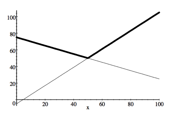
The objective is to minimize the total cost: \(\max\left\{ (c-b)x+bd, (c+h)x-hd\right\}\). For example, suppose we have \(c=1\), \(b=1.5\), \(h=0.1\), and \(d=50\). Then the following figure illustrates the total cost:
In general, the ordering decision is made before a realization of the demand is known. The deterministic formulation corresponds to a single scenario taken with probability one:
Now suppose we model the distribution of possible demands with scenarios \(d_1, \ldots, d_K\) each with equal probability (\(p_k = 0.2\)). Then the following formulation minimizes the expected value of the total cost over these scenarios:
This is a linear problem, so it can be formulated with SimpleModel, PuLP and Pyomo.
Since the two constraints are indexed from \(1, \ldots, K\), we can group them together into a single block, which itself is indexed from \(1, \ldots, K\).
Below, we show formulations for SimpleModel, PuLP, and Pyomo. The SimpleModel and PuLP models illustrate unstructured representations. The first Pyomo formulation illustrates an unstructured representation, where constraints are stored in a list. The second Pyomo formulation illustrates a structured representation, which corresponds to the first formulation above. The final Pyomo formulation illustrates a hierarchical representation, using the Block component to structure the model representation in a modular manner.
SimpleModel Formulation
The following script creates and solves a linear program for the newsvendor problem using SimpleModel:
1 2 3 4 5 6 7 8 9 10 11 12 13 14 15 16 17 18 19 20 21 22 23 24 25 26 27 28 29 30 | # newsvendor.py
from pyomo_simplemodel import *
c=1.0
b=1.5
h=0.1
d = {1:15, 2:60, 3:72, 4:78, 5:82}
scenarios = range(1,6)
m = SimpleModel()
x = m.var('x', within=NonNegativeReals)
y = m.var('y', scenarios)
for i in scenarios:
m += y[i] >= (c-b)*x + b*d[i]
m += y[i] >= (c+h)*x - h*d[i]
m += sum(y[i] for i in scenarios)/5.0
status = m.solve("glpk")
print("Status = %s" % status.solver.termination_condition)
print("%s = %f" % (x, value(x)))
for i in y:
print("%s = %f" % (y[i], value(y[i])))
print("Objective = %f" % value(m.objective()))
|
There are two key things to note about this model. First, the model
simply consists of a list of constraints. Second, the y variable
is indexed to represent the total cost for the different scenarios.
PuLP Formulation
The following script creates and solves a linear program for the newsvendor problem using PuLP:
1 2 3 4 5 6 7 8 9 10 11 12 13 14 15 16 17 18 19 20 21 22 23 24 25 26 27 28 29 30 31 | # newsvendor-pulp.py
from pulp import *
c=1.0
b=1.5
h=0.1
d = {1:15, 2:60, 3:72, 4:78, 5:82}
scenarios = range(1,6)
M = LpProblem("Newsvendor")
x = LpVariable('x', lowBound=0)
y = LpVariable.dicts('y', scenarios)
for i in scenarios:
M += y[i] >= (c-b)*x + b*d[i]
M += y[i] >= (c+h)*x - h*d[i]
M += sum(y[i] for i in scenarios)/5.0
M.solve()
print("Status = %s" % LpStatus[M.status])
print("%s = %f" % (x.name, value(x.varValue)))
for i in scenarios:
print("%s = %f" % (y[i].name, y[i].varValue))
print("Objective = %f" % value(M.objective))
|
As with the SimpleModel formulation, the model consists of a list
of constraints, and the y variable is indexed.
Pyomo Formulations
The following script creates and solves a linear program for the newsvendor problem using Pyomo:
# newsvendor-pyomo1.py

from pyomo.environ import *

c=1.0
b=1.5
h=0.1
d = {1:15, 2:60, 3:72, 4:78, 5:82}

scenarios = range(1,6)

M = ConcreteModel()
M.x = Var(within=NonNegativeReals)
M.y = Var(scenarios)

M.c = ConstraintList()
for i in scenarios:
  M.c.add( M.y[i] >= (c-b)*M.x + b*d[i] )
  M.c.add( M.y[i] >= (c+h)*M.x - h*d[i] )

M.o = Objective(expr=sum(M.y[i] for i in scenarios)/5.0)

solver = SolverFactory('glpk')
status = solver.solve(M)

print("Status = %s" % status.solver.termination_condition)

print("%s = %f" % (M.x, value(M.x)))
for i in scenarios:
    print("%s = %f" % (M.y[i], value(M.y[i])))
print("Objective = %f" % value(M.o))
This model uses the ConstraintList component to store a list of constraints, and the y variable
is indexed. Thus, this model provides an unstructured representation that is similar to models generated with SimpleModel and PuLP.
The following script uses Pyomo to create and solve the newsvendor problem, using a structured representation:
# newsvendor-pyomo2.py

from pyomo.environ import *

c=1.0
b=1.5
h=0.1
d = {1:15, 2:60, 3:72, 4:78, 5:82}

scenarios = range(1,6)

M = ConcreteModel()
M.x = Var(within=NonNegativeReals)
M.y = Var(scenarios)

def greater_rule(M, i):
  return M.y[i] >= (c-b)*M.x + b*d[i]
M.greater = Constraint(scenarios, rule=greater_rule)

def less_rule(M, i):
  return M.y[i] >= (c+h)*M.x - h*d[i]
M.less = Constraint(scenarios, rule=less_rule)

def o_rule(M):
    return sum(M.y[i] for i in scenarios)/5.0
M.o = Objective(rule=o_rule)

solver = SolverFactory('glpk')
status = solver.solve(M)

print("Status = %s" % status.solver.termination_condition)

print("%s = %f" % (M.x, value(M.x)))
for i in scenarios:
    print("%s = %f" % (M.y[i], value(M.y[i])))
print("Objective = %f" % value(M.o))
The named constraint components greater and less define
two groups of constraints for the model, each of which has the same
mathematical form. These named components provide a structured
representation for these constraints.
Finally, the following script uses Pyomo to create and solve this problem, using a hierarchical representation:
# newsvendor-pyomo3.py

from pyomo.environ import *

c=1.0
b=1.5
h=0.1
d = {1:15, 2:60, 3:72, 4:78, 5:82}

scenarios = range(1,6)

M = ConcreteModel()
M.x = Var(within=NonNegativeReals)

def b_rule(B, i):
  B.y = Var()
  B.greater = Constraint(expr=B.y >= (c-b)*M.x + b*d[i])
  B.less    = Constraint(expr=B.y >= (c+h)*M.x - h*d[i])
  return B
M.b = Block(scenarios, rule=b_rule)

def o_rule(M):
    return sum(M.b[i].y for i in scenarios)/5.0
M.o = Objective(rule=o_rule)

solver = SolverFactory('glpk')
status = solver.solve(M)

print("Status = %s" % status.solver.termination_condition)

print("%s = %f" % (M.x, value(M.x)))
for i in scenarios:
    print("%s = %f" % (M.b[i].y, value(M.b[i].y)))
print("Objective = %f" % value(M.o))
A block is added for each index \(k =
1,\ldots,K\). Each block contains a variable y, and the
corresponding constraints that define the value of y.
Note that the block component b is indexed in this formulation
while the y variable is indexed in the other formulations above.
Block components allow Pyomo to support a modular modeling framework
where data, variables and constraints can be
represented together for each index value. There
are several advantages of this approach:
- This model structure is explicit, and it can be exploited by decomposition-based optimization solvers (e.g. the progressive hedging solver in Pyomo).
- Extending and refining models is simpler with blocks. For example, if a multi-dimensional index was needed for this problem, then only the block
bwould need to be modified to reflect that.
| [ShaPhi] |
|